P-Y Curves for Laterally Loaded Piles
P-Y curves are the numerical models used to simulate the response of soil resistance (p, soil resistance per unit length of the pile) to the pile deflection (y) for the piles under lateral loading. With this approach, the soils are conveniently represented by a series of nonlinear springs varying with the depth and soil type in the analysis for laterally loaded piles.
This concept was first developed in the 1940’s and 1950’s when energy companies built offshore structures that had to sustain heavy horizontal loads from waves. An exact publication date of the model is not available since the p-y curves are still modified and improved today. The earliest recommendations on p-y curves could be traced back to the 1950s by the works of Skempton and Terzaghi (Ruigrok 2010).
Ideally, p-y curves should be generated from full-scale lateral load tests on instrumented test piles. In the absence of experimentally derived p-y curves, it is possible to use empirical p-y formulations that have been proposed in the literature for different types of soils.
From the 1970s, Further modification and improvement have been given to the p-y method. Instead of giving inputs for the nonlinear spring constant (i.e., the values of the spring constant as a function of pile deflection), p-y curves are given as inputs to the analysis in the p-y method. Different p-y curves have been developed over the years for different soil types, which give the magnitude of soil pressure as a function of the pile deflection.
In the analysis, the pile is divided into small segments, and for each segment, a p-y curve is given as input. Depending on the magnitude of the deflection of a pile segment, the correct soil resistance is calculated from the p-y curve iteratively. With the development of the finite element method, analysis using beam finite elements has been widely adopted in many calculations involving the subgrade-reaction approach or the p-y method. Today, the p-y method is the most widely used method for calculating the response of laterally loaded piles.

P-Y Curve Models in PileLAT and PileGroup Programs
Cohesive Soils
There are five different P-Y curves available for modeling cohesive soils:
-
API Clay RP2A. API Clay RP2A (2000) is the p-y curve model for soft clay recommended in API RP2A 21st Edition (2000), where the ultimate resistance (Pu) of soft clay is determined in the same way as Matlock (1970).
-
API Clay RP2GEO. API soft clay p-y curve model is further updated in API RP 2GEO 1st Edition (2014), The only difference from API Clay RP2A (2000) model is that more controlling points are added to the piece-wise curves as shown in the figures below for both static and cyclic loading conditions.
-
Soft Clay (Matlock). This is based on the method established by Matlock (1970) for both static and cyclic loading conditions.
-
Stiff Clay without Water (Reese). This p-y curve model for still clay without water is based on the works by Welch and Reese (1972).
-
Stiff Clay without Water with Initial Modulus. This p-y curve model is based on the works of Welch and Reese (1972) except the initial slope follows the recommendations on the model of still clay with water by Reese et al. (1975).
-
Stiff Clay with Water (Reese). This p-y curve model is based on the works by Reese et al. (1975) where the lateral ultimate resistance is determined separately for the location near the ground surface and also at a deep depth
-
Cemented c-phi soil (Silt). The P-y curve for cemented c-phi soil (Silt) is based on the recommendation by Evans and Duncan (1982) and Reese and Impe (2010).
-
Non-liquefied Crust for Cohesive Soils (NZTA 553). This p--y curve model is based on the recommendations from NZ Transport Agency research report (NZTA) 553 dated July 2014.
-
Piedmont Residual Soil - Simpson and Brown (2003). This p-y curve model is Piedmont residual soils under lateral loading.
Cohesionless Soils
There are three different P-Y curves available for modeling cohesionless soils:
-
API Sand. The p-y curve model follows the recommendations in API RP 2GEO 1st Edition (2014).
-
Reese Sand. The p-y curve model is based on the works of Reese et al. (1974) for both static and cyclic loading conditions.
-
Liquefied Sand. The p-y curve model is based on the works of Rollins et al. (2005).
-
Calcareous Soil - Dyson and Randolph (2001). The p-y curve model is based on the recommendation by Dyson and Randolph (2001).
-
Calcareous Soil - Novello (1999). The p-y curve model is based on the recommendation by Novello (1999).
-
Non-liquefied Cohesionless soils (NZTA 553). This p--y curve model is based on the recommendations from NZ Transport Agency research report (NZTA) 553 dated July 2014.
-
Liquefied Soils (NZTA 553). This p--y curve model is based on the recommendations from NZ Transport Agency research report (NZTA) 553 dated July 2014.
-
Sand - Kallehave et al. (2012). This p-y curve model is an empirical approach designed to predict the lateral response of piles in sandy soils. It addresses the limitations of the API Sand method (American Petroleum Institute), which is often inadequate for large-diameter piles, such as those used in offshore wind turbine monopiles.
-
Sand - Sorensen et al. (2010). This p-y curve model is for assessing the lateral response of large diameter monopiles embedded in sandy soils. This model emerged from the need to improve the accuracy of lateral load predictions for large-diameter monopiles, especially in the context of offshore structures, where traditional p-y models often fell short.
-
Sand - Suryasentana and Lehane (2014). This p-y curve model provides an enhanced method for predicting the lateral response of piles in sandy soils, particularly addressing the behavior of large-diameter piles used in offshore wind turbine foundations, based on in-situ cone penetration testing (CPT) results.
-
Small Strain Sand - Hanssen (2015). This p-y curve model is a modification of the p-y curves as recommended in API-RP-2A for sand, with using a small strain overly to the original curves to accommodate design with site specific soil parameters instead of empirical correlations.
-
Loess Soil - Johnson et al. (2007). This p-y curve model is for piles in loess soil presents unique challenges due to the distinct characteristics of loess, such as its loose structure, collapsibility, and high susceptibility to settlement when subjected to moisture.
-
Hybrid Liquefied Sand - Franke & Rollins (2013). This p-y curve model is based on the works of Franke and Rollins (2013) where the p-y curve based on Rollins et al. (2005) for liquefied sand is combined with the p-y curve from Matlock (1970) for soft clays under static loading where the soil strength is based on residual strength of liquefied soils.
Rock
There are four different P-Y curves available for modeling rock:
-
Weak Rock - Reese (1997). The p-y curve model is based on the method established by Reese (1997).
-
Strong Rock - Turner (2006). The p-y curve for strong rock is based on the method proposed by Turner (2006).
-
Massive Rock - Liang et al. (2009). The p-y curve for massive rock is based on the method proposed by Liang et al. (2009).
-
Calcareous Rock - Fragio et al. (1985). The p-y curve for calcareous rocks is based on the method proposed by Fragio et al. (1985).
-
Weak Carbonate Rock - Abbs (1983). The P-y curve for weak carbonate rock was developed by Abbs (1983) for offshore platforms in the Middle East with carbonate rocks having unconfined compressive strength in the range from 0.5 to 5 MPa.
General Geotechnical Materials
There are two options available for modeling the general geotechnical materials:
-
Elastic-Plastic Model. The soil subgrade modulus is determined by Vesic's method and the ultimate lateral resistance is determined by API clay model for cohesive soils, Reese sand model for granular soils and Weak rock - Reese method for rocks.
-
Elastic Model. The elastic subgrade modulus is adopted in the method.
-
User-defined Model. The p-y curve model can be defined by the users.
API Clay RP2A (2000)
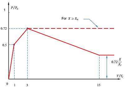
API Clay RP2A (2000) is the p-y curve model for soft clay recommended in API RP2A 21st Edition (2000), where the ultimate resistance (Pu) of soft clay is determined in the same way as Matlock (1970). The only difference from Matlock soft clay model is that the piece-wise curves are used as shown in the figures below for both static and cyclic loading conditions. More information can be found here.
.png)
P-Y curve under static loading condition
%20Cyclic.png)
P-Y curve under cyclic loading condition
API Clay RP2GEO (2014)
API soft clay p-y curve model is further updated in API RP 2GEO 1st Edition (2014), where the ultimate resistance (Pu) of soft clay is determined in the same way as Matlock (1970). The only difference from API Clay RP2A (2000) model is that more controlling points are added to the piece-wise curves as shown in the figures below for both static and cyclic loading conditions. More information can be found here.
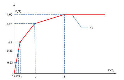
P-Y curve under static loading condition
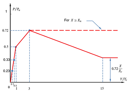
P-Y curve under cyclic loading condition
Soft clay (Matlock) model
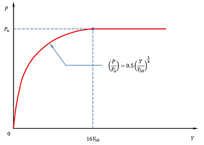
P-Y curves for soft clay with water based on the method established by Matlock (1970) are shown below for both static and cyclic loading conditions.

P-Y curve under static loading condition

P-Y curve under cyclic loading condition
Stiff Clay without Water
The following figures show the P-Y curves for stiff clay without water based on Welch and Reese (1972) under both static and cyclic loading conditions.
P-Y curve under static loading condition
P-Y curve under cyclic loading condition
Stiff Clay without Water with initial subgrade modulus
This model is similar to stiff clay without water based on the method by Welch and Reese (1972) except for that the initial slope follows the recommendations on the model of stiff clay with water by Reese et al. (1975).
The initial straight-line portion of the P-Y curve is calculated by multiplying the depth, X by Ks. The values of Ks are determined based on the values of undrained shear strength as follows (Reese and Van Impe, 2001)

P-Y curve under static loading condition
Stiff Clay with Water
P-Y curves for stiff clay with water are based on the method established by Reese et al. (1975) under both static and cyclic loading conditions.
P-Y curve under static loading condition
P-Y curve under cyclic loading condition
Cemented c-phi Soil
P-Y curves for cemented c-phi soil are based on the recommendation by Reese and Van Impe (2011). More details can be found from this page.
P-Y curve for cemented c-phi soil
Non-liquefied Crust for Cohesive Soils - NZTA 553
P-Y curves for non-liquefied crust for cohesive soils are based on the recommendation from NZ Transport Agency research report 553 - the development of design guidance for bridges in New Zealand for liquefaction and lateral spreading effects published in 2014. More details can be found from this page.
P-Y curve for non-liquefied crust for cohesive soils - NZTA 553
Piedmont Residual Soil - Simpson and Brown (2003)
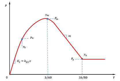
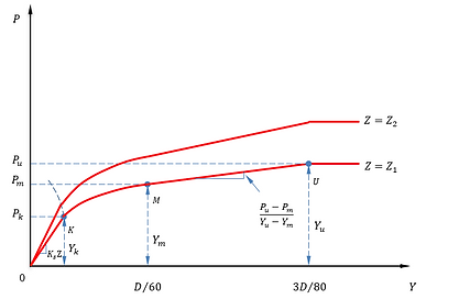
P-Y curves for piedmont residual soil are based on the recommendation from Simpson and Brown (2003). More details can be found from this page.
P-Y curve for piedmont residual soils - Simpson and Brown (2003)
Reese Sand
P-Y curves for sand based on Reese et al. (1974) for both static and cyclic loading conditions are shown in the figure below. More details can be found from this page.
P-Y curve for Reese Sand model under both static and cyclic loading condition
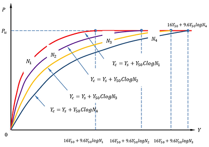
Liquefied Sand - Rollins et al. (2005)
P-Y curves for liquefied sand is based on the works of Rollins et al. (2005) and is shown in the figure below. More details can be found from this page.
P-Y curve for Liquefied Sand
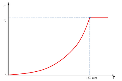
Calcareous Soil - Dyson and Randolph (2001)
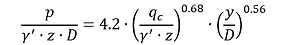
P-Y curve for calcareous soils has a markedly different format to those for sand and clay. This unique response was identified in centrifuge modelling undertaken in the late 1980s at Cambridge University. The p-y curve is based on the recommendation by Dyson and Randolph (2001) and given by the following relationship:
Note that γ' is effective unit weight of the soil, D is the pile width/diameter, R is the constant for curve stiffness (typical value = 2.7), qc is cone penetration resistance at the node depth, n is the empirical constant (typical value = 0.72), and m is the constant for p-y curve curvature (typical value = 0.58). The figure below shows the typical p-y curve based on Dyson and Randolph (2001).
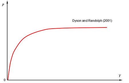
P-Y curve for Calcareous Soil - Dyson and Randolph (2001)
Calcareous Soil - Novello (1999)
P-Y curve for calcareous soils is based on the recommendation by Novello (1999) and given by the following relationship:
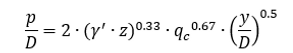
Note that γ' is effective unit weight of the soil, D is the pile width/diameter, Z is the point below the ground surface and qc is cone penetration resistance at the node depth. The figure below shows the typical p-y curve based on Novello (1999).

P-Y curve for Calcareous Soil - Novello (1999)
Sand - Kallehave et al. (2012)
The p-y curve model by Kallehave et al. (2012) is an empirical approach designed to predict the lateral response of piles in sandy soils. It addresses the limitations of the API Sand method (American Petroleum Institute), which is often inadequate for large-diameter piles, such as those used in offshore wind turbine monopiles. The Kallehave et al. (2012) model is based on API Sand – API (2014) for determining ultimate lateral resistance, but introduces a modification to the subgrade reaction modulus (K x Z in the equation below) as shown in the equation below:
where Z0 = 2.5 m and D0 = 0.61 m.
The lateral soil resistance-deflection (P-Y) relationship is described by the equation below, similar to API Sand – API (2014):
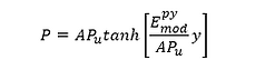
where:
P = Actual lateral resistance
A = Factor to account for cyclic or static loading conditions (0.9 for cyclic loading, max for static loading)
z = Depth below the ground surface
k = Rate of increase with depth of initial modulus of subgrade reaction which can be determined from API RP 2GEO 1st Edition (2014).
y = lateral deflection
Pu = ultimate lateral resistance
Sand - Sorensen et al. (2010)
The p-y curve model of Sorensen et al. (2010) provides a similar approach for assessing the lateral response of large diameter monopiles embedded in sandy soils. This model emerged from the need to improve the accuracy of lateral load predictions for large-diameter monopiles, especially in the context of offshore structures, where traditional p-y models often fell short. The Sorensen et al. (2010) model is based on API Sand – API (2014) for determining ultimate lateral resistance, but introduces a modification to the subgrade reaction modulus (K x Z in the equation below) as shown in the equation below:
where Zref = 1.0 m, Dref = 1.0 m, α = 50000 kN/m^2, φ is effective friction angle (in radians) and d=3.6.
The lateral soil resistance-deflection (P-Y) relationship is described by the equation below, similar to API Sand – API (2014):
where:
P = Actual lateral resistance
A = Factor to account for cyclic or static loading conditions (0.9 for cyclic loading, max for static loading)
z = Depth below the ground surface
k = Rate of increase with depth of initial modulus of subgrade reaction which can be determined from API RP 2GEO 1st Edition (2014).
y = lateral deflection
Pu = ultimate lateral resistance
Sand - Suryasentana and Lehane (2014)
The p-y curve model developed by Suryasentana and Lehane (2014) provides an enhanced method for predicting the lateral response of piles in sandy soils, particularly addressing the behavior of large-diameter piles used in offshore wind turbine foundations, based on in-situ cone penetration testing (CPT) results. The p-y curve is based on equation below:
Note that γ' is effective unit weight of the soil, D is the pile width/diameter, Z is the point below the ground surface and qc is cone penetration resistance at the node depth. The figure below shows the typical p-y curve Suryasentana and Lehane (2014).

P-Y curve for Sand - Suryasentana and Lehane (2014)
Small Strain Sand - Hanssen (2015)
Hanssen (2015) proposed a modification of the p-y curves as recommended in API-RP-2A for sand, with using a small strain overly to the original curves to accommodate design with site specific soil parameters instead of empirical correlations.
The p-y curves for small strain sand proposed by Hanssen (2015) provide an improved method for analyzing the lateral response of piles embedded in sand, especially at low strain levels. Traditional p-y curves, typically used in geotechnical engineering to model soil-pile interaction, often lack accuracy at small strains, where soil stiffness can vary significantly. Hanssen’s approach aims to address this limitation by incorporating the effects of small strain stiffness, leading to a more realistic representation of the soil response under lateral loading.
In Hanssen’s (2015) model, the nonlinearity of the soil behavior at small strains is explicitly considered, which enhances the prediction of both pile deflections and bending moments, particularly for structures subjected to repeated or cyclic loading. This is critical in cases where high sensitivity to initial soil stiffness could influence design decisions, such as in offshore structures or other critical infrastructure with high lateral load demands.
The p-y curve is based on the equations below:
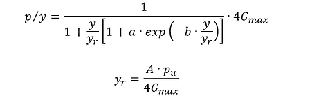
where:
P = Actual lateral resistance
A = Factor to account for cyclic or static loading conditions (0.9 for cyclic loading, max for static loading)
yr = Reference displacement
y = lateral deflection
Pu = ultimate lateral resistance
a = Empirical constant
b = Empirical constant. This value is adopted to be 1 as per Wichtmann and Triantafyllidis (2010).
Gmax = Shear stiffness at small strains.
Hanssen (2015) adopted the following empirical relationship to calculate the shear stiffness at small strains (Gmax):
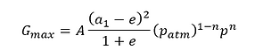
The empirical constants in the equations above can be selected based on the relationships summarised below (Hanssen 2015):

where Cu is the coefficient of uniformity.

P-Y curve for Small Strain Sand – Hanssen (2015)
Loess Soil – Johnson et al. (2007)
The lateral response of piles in loess soil presents unique challenges due to the distinct characteristics of loess, such as its loose structure, collapsibility, and high susceptibility to settlement when subjected to moisture. Traditional p-y curve models, which describe the relationship between lateral soil resistance (p) and lateral pile displacement (y), are generally derived from more consolidated soil types, such as sand or clay. These models often fall short of accurately predicting pile behaviour in loess, where the soil structure is prone to rapid degradation under loading.
Johnson et al. (2007) recognized these limitations and developed a specialized p-y curve model tailored specifically to loess soils. Their model incorporates the unique stress-strain behaviour of loess, acknowledging its rapid stiffness reduction and the impact of soil moisture and density on lateral resistance. By conducting field and laboratory tests, they calibrated empirical relationships that reflect the characteristic behaviour of loess, particularly under varying levels of saturation.
The Johnson et al. (2007) p-y model for loess soil allows engineers to more accurately predict pile deflections, bending moments, and lateral resistance, enhancing the reliability of pile foundation designs in regions with extensive loess deposits. This model is especially relevant for geotechnical projects where the performance of laterally loaded piles in loess soils is critical to structural stability and serviceability. P-Y curves for loess soil based on Johnson et al. (2007) and are shown in the figure below.
P-Y curve for Loess Soil - Johnson et al. (2007)
The p-y curve is based on the equations below:
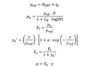
where:
NCPT = Cone bearing capacity factor
qc = Cone tip resistance
pu0 = Ultimate unit lateral soil resistance based on cone top resistance
D = Pile diameter
CN = Dimensionless constant for cyclic effect. This value is adopted to be 0.24
N = Number of cycles for cyclic loading. For static loading, the value is equal to 1.
Pu = Ultimate lateral soil resistance
yref = Reference displacement. This value is adopted to be 0.117 inches or 0.0029718 meters as per Johnson et al. (2007)
α = Dimensionless constant (=0.1)
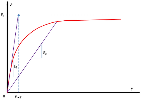
yh' = Hyperbolic function of the reference displacement and lateral pile displacement
Ei = Initial modulus
Es = Secant modulus
y = Lateral pile displacement
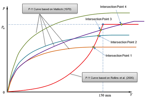
Hybrid Liquefied Sand – Franke & Rollins (2013), Wang & Reese (1998)
P-Y curves for hybrid liquefied sand is based on the works of Franke and Rollins (2013) where the p-y curve based on Rollins et al. (2005) for liquefied sand is combined with the p-y curve from Matlock (1970) for soft clays under static loading where the soil strength is based on residual strength of liquefied soils. The lower lateral resistance from those curves is considered in the analysis. The four possible combinations of the p-y curves are shown in the figure below.
P-Y curve for Loess Soil - Johnson et al. (2007)
The p-y curve is based on the equations below:
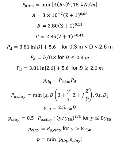
where:
A, B and C are dimensionless functions of the depth (Z) of the curve in meters
Z is depth below the ground surface
y is pile lateral deflection
D is pile diameter
P0.3m is the maximum dilative resistance for a 0.3 m diameter pile
Pd is a dimensionless factor to adjust for pile diameter
pliq is ultimate lateral resistance based on Rollins et al. (2005)
sr is residual soil strength
γ' is average effective unit weight used to calculate the effective overburn stress
ε50 is the strain factor which is the strain measured at one-half the maximum stress for an undrained tri-axial compression test
y50 is the reference displacement
Pu,clay is ultimate lateral resistance calculated based on the method by Matlock (1970)
Pclay is lateral resistance calculated for a specific pile deflection y based on Matlock (1970)
pliq is lateral resistance calculated for a specific pile deflection y based on Rollins et al. (2005)
p is actual lateral resistance
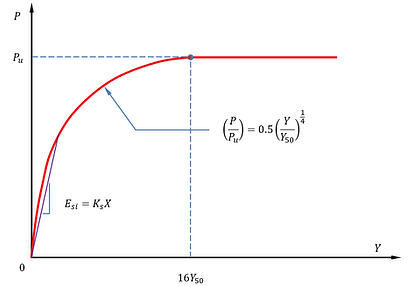
Weak Rock - Reese (1997)
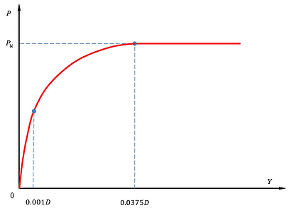
P-Y curves for weak rock are calculated using the method established by Reese (1997) and shown in the figure below.
P-Y curve for Weak Rock - Reese (1997)
More information for this p-y curve model can be found from the technical blog here.
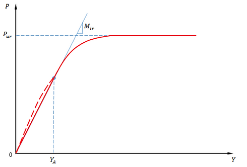
Strong Rock - Tunner (2006)
P-Y curves for strong rock are calculated using the method by Turner (2006) and are shown in the figure below.
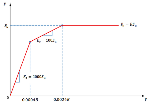
P-Y curve for strong rock - Tunner (2006)
The ultimate resistance of strong rock is given by the following equation:
where:
B is pile diameter
Pu is ultimate lateral resistance
su is the half of the unconfined compressive strength (UCS) of the strong rock